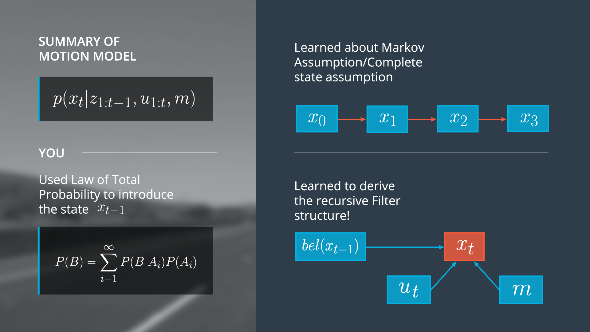
20. Recursive Structure

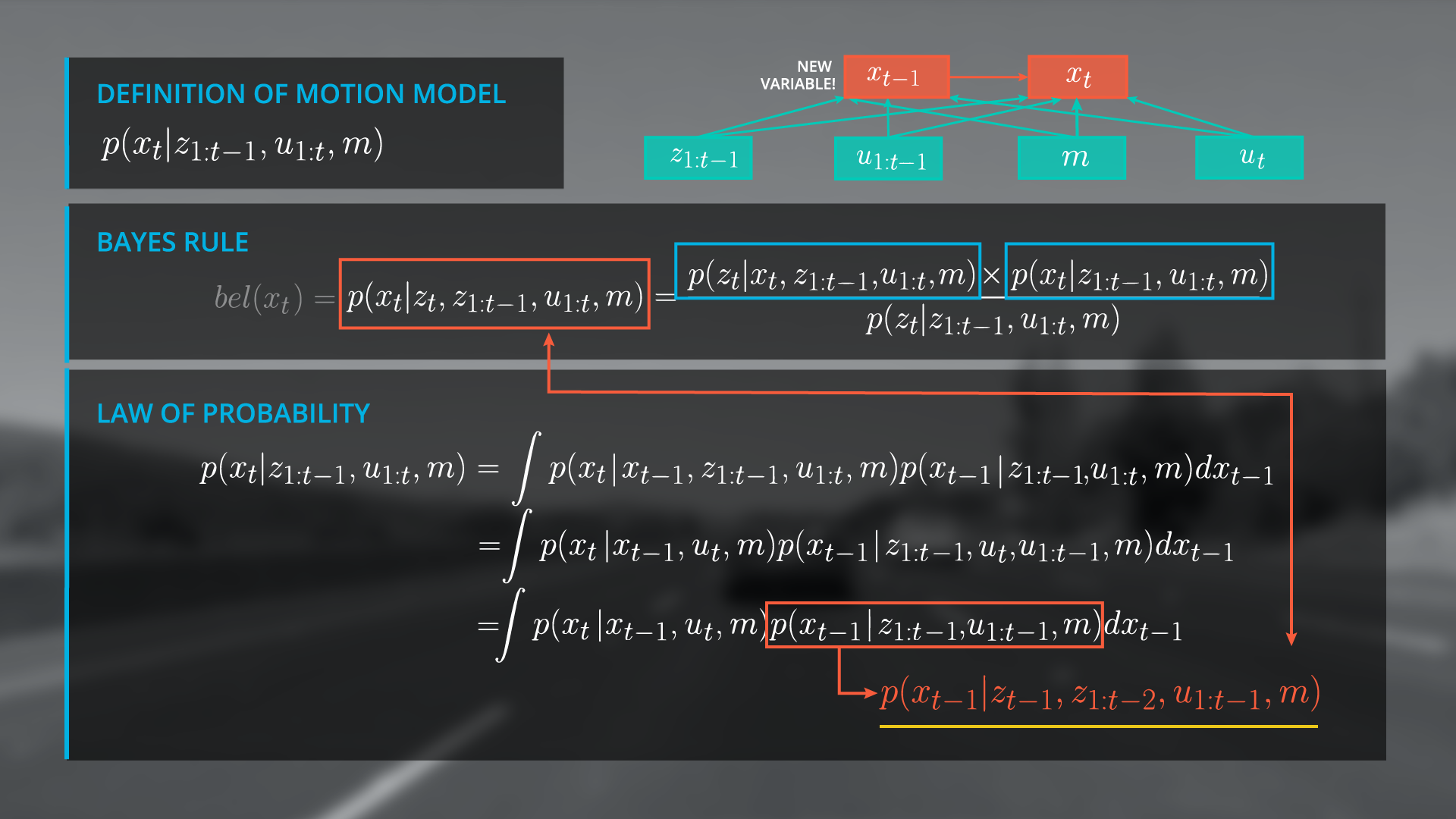
We have achieved a very important step towards the final form of our recursive state estimator. Let’s see why. If we rewrite the second term in our integral to split z_{1-t} to z_{t-1} and z_{t-2} we arrive at a function that is exactly the belief from the previous time step, namely bel(x_{t-1}) .

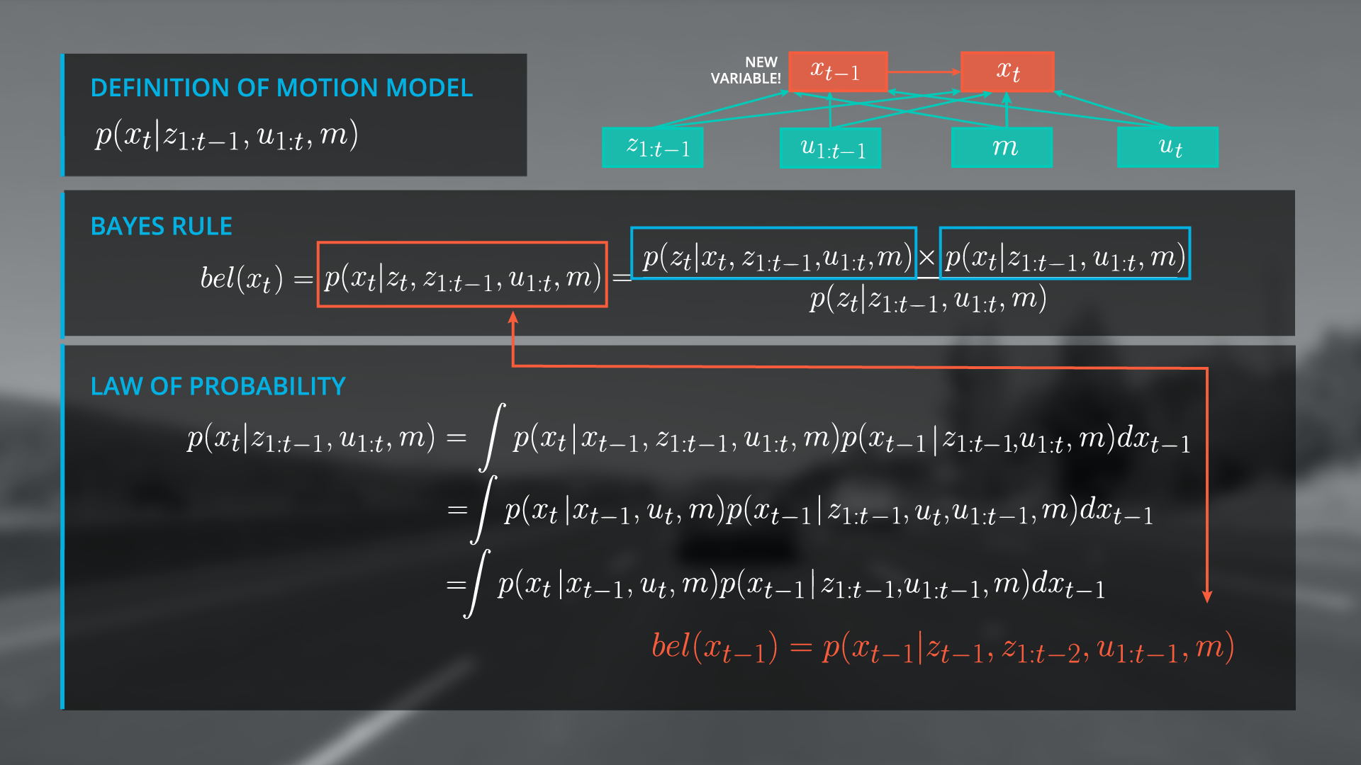
Now we can rewrite out integral as the belief of x_{t-1} .

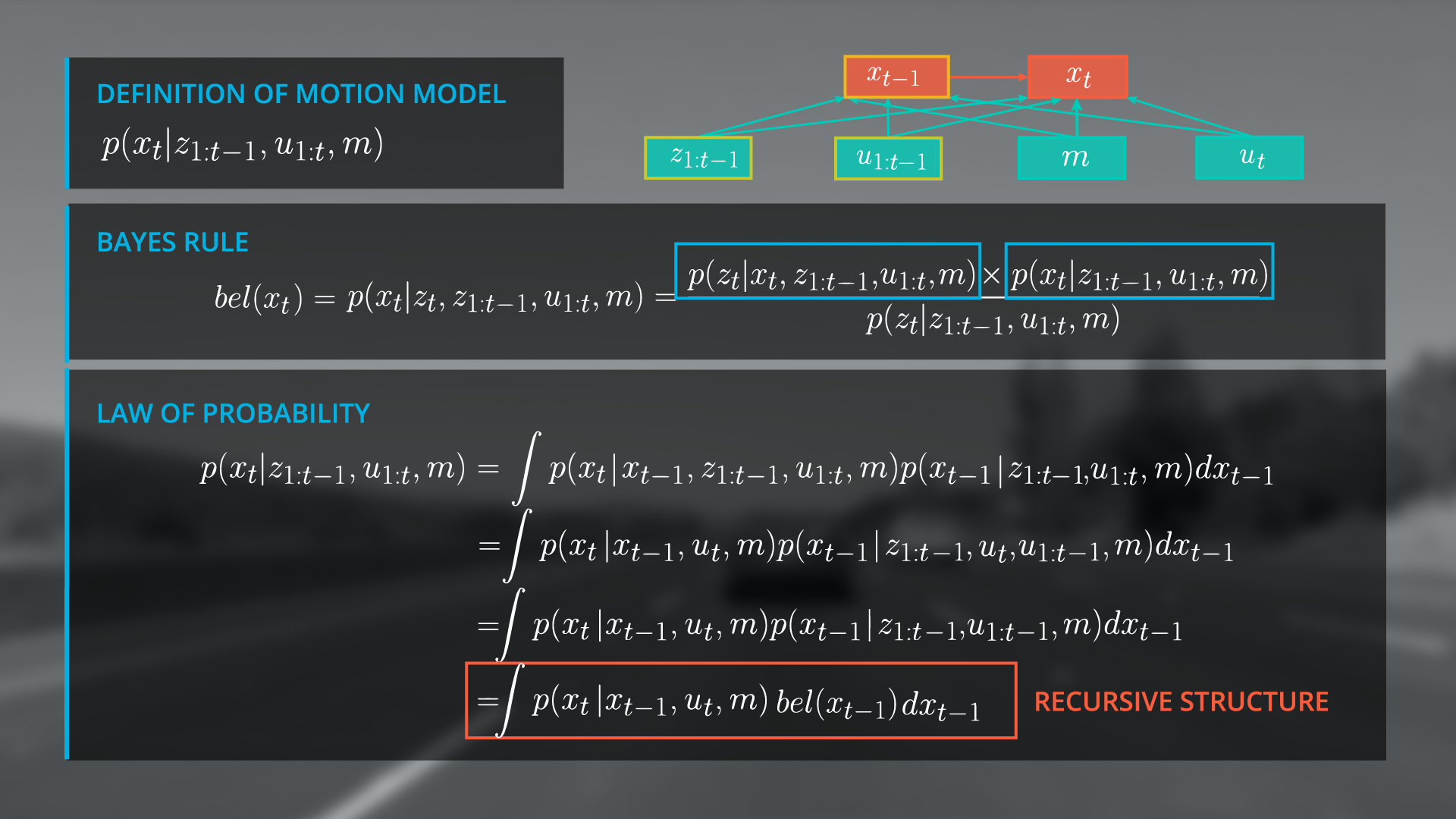
The amazing thing is that we have a recursive update formula and can now use the estimated state from the previous time step to predict the current state at t. This is a critical step in a recursive Bayesian filter because it renders us independent from the entire observation and control history. So in the graph structure, we will replace the previous state terms (highlighted) with our belief of the state at x at t-1 (next image).

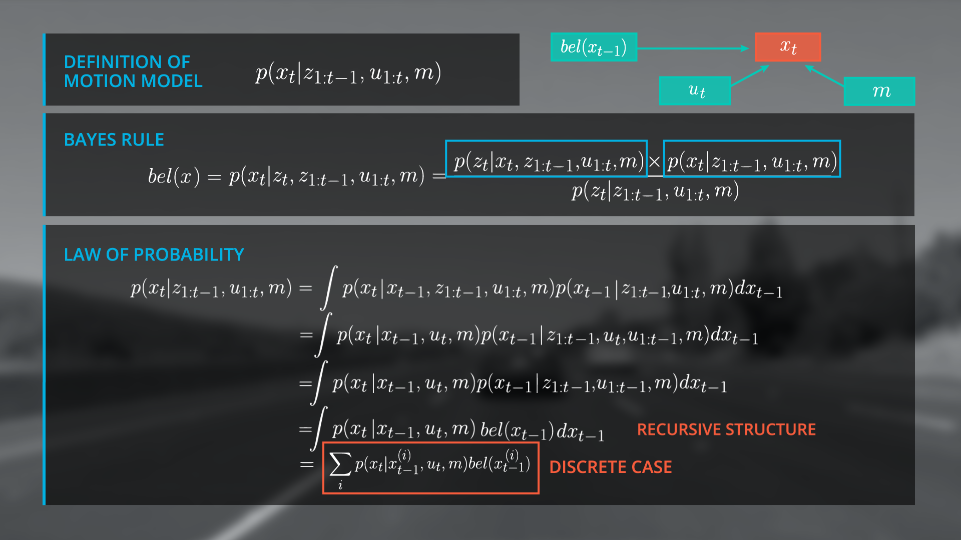
Finally, we replace the integral by a sum over all x_i because we have a discrete localization scenario in this case, to get the same formula in Sebastian's lesson for localization. The process of predicting x_t with a previous beliefs ( x_{t-1} ) and the transition model is technically a convolution. If you take a look to the formula again, it is essential that the belief at x_t = 0 is initialized with a meaningful assumption. It depends on the localization scenario how you set the belief or in other words, how you initialize your filter. For example, you can use GPS to get a coarse estimate of your location.